3.3. Conservation, area corrections and accumulation
Conservation of mass and energy is a defining requirement of the mediator: a flux leaving one component must deposit the same integrated quantity in the component that receives it, even after being mapped and merged across mismatched grids and averaged over mismatched coupling intervals. Achieving this ties together several details that must be considered together — mapping weights, surface fractions, normalization, model-versus-ESMF areas, and accumulation.
CMEPS’s mapping weights are pure area-overlap weights: each is the fractional area a source cell contributes to a destination cell. Masking and normalization are deliberately not folded into them. The reason is a split between the static and the dynamic:
the weights are static geometry — area overlaps between cells, computed once and reused every coupling step, and summing to one; whereas
the masking and normalization are dynamic — they are done with the ocean/ice surface fraction, which changes in time as sea ice grows and melts (the ocean fraction is
1 - ice fraction).
A time-varying fraction cannot be precomputed into static weights, so it is applied at run time, every coupling step, when a field is mapped or merged: a partial-coverage field is fraction-weighted and normalized when mapped, and the surface contributions are fraction-weighted when merged. (ESMF could fold a static land/ocean mask into the weights, but that static mask cannot represent the dynamic ice coverage that conservation depends on, and folding normalization in would break the sum-to-one property besides.)
This page develops why that combination conserves; it is the principle that the Mapping, Merging and fractions pages that follow then implement, and it expands the conservation summary in Core concepts.
The example below uses a single atmosphere cell a that overlaps four
ocean/ice cells 1..4; A is an overlap area, w a mapping weight, f
a surface fraction, F a field, and subscripts l/o/i denote land, ocean
and ice.
The figures below make this setup concrete. In the most common CMEPS configuration the ocean and sea-ice grids are identical, as are the atmosphere and land grids, and the ocean/ice grid carries the mask that distinguishes ocean/ice cells from land.
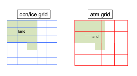
Overlapping atmosphere and ocean/ice grids. Interpolating the ocean/ice mask onto the atmosphere/land grid sets the complementary land and ocean/ice masks there; the land model may make a single atmosphere cell part land, part ocean and part sea ice.
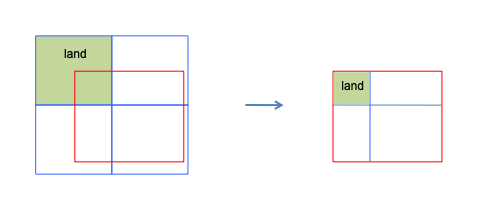
Focusing on a single atmosphere cell a and the ocean/ice cells 1..4
it overlaps.
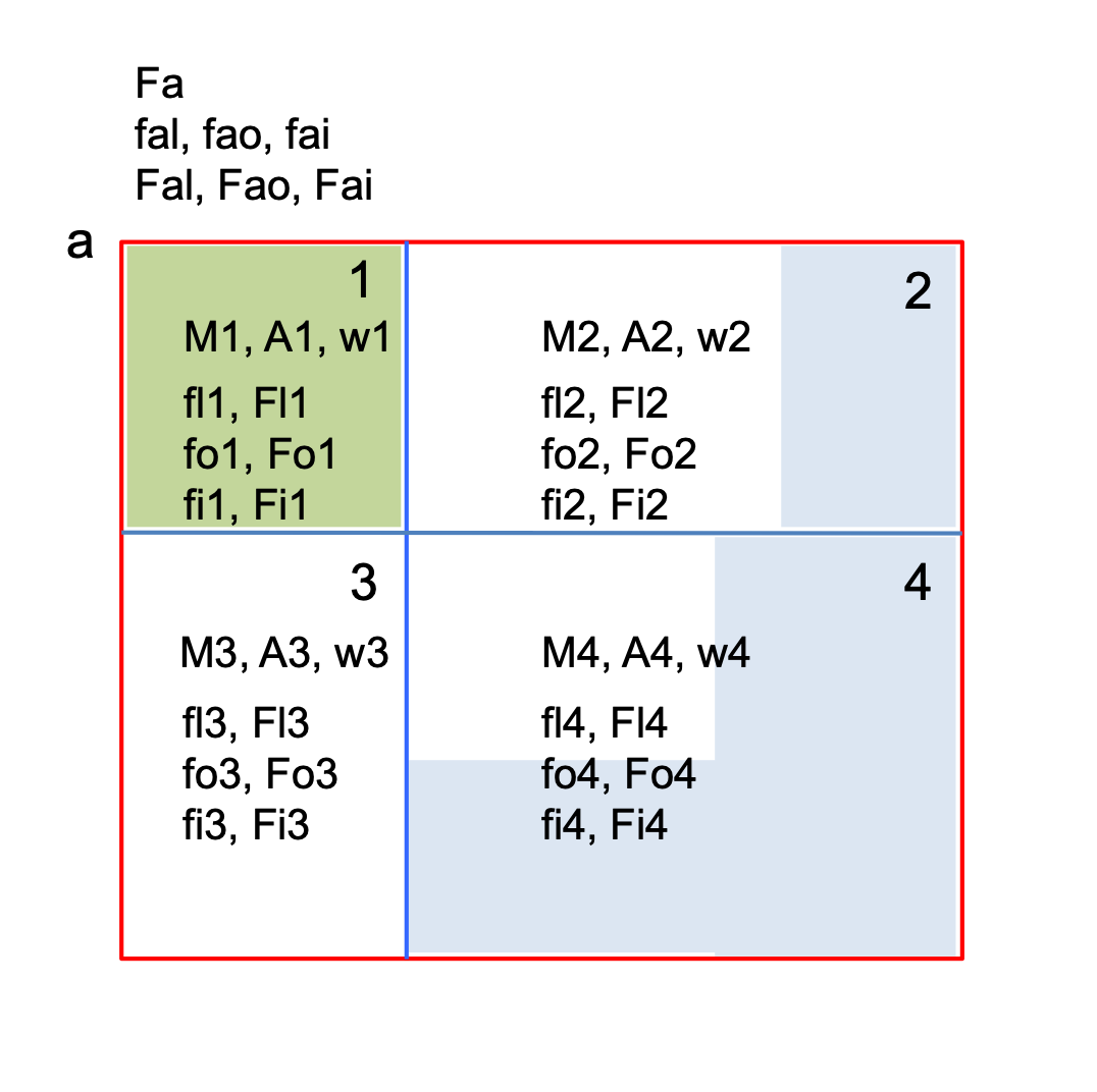
The labeling used throughout this page. Each overlap i has an area Ai
and a mask Mi (land green, ocean blue, sea ice white). On the atmosphere
cell the land, ocean and ice fractions satisfy fal + fao + fai = 1, and
Fa is the merged gridcell-average field.
3.3.1. Conservative mapping weights
CMEPS uses area-overlap conservative weights,
w1 = A1/Aa, w2 = A2/Aa, w3 = A3/Aa, w4 = A4/Aa
which, being fractions of the atmosphere cell area, always sum to one:
w1 + w2 + w3 + w4 = 1
Applying the weights is a sparse matrix multiply, Xa = [W] Xo. These same
weights map the ocean/ice mask to obtain the land fraction, and map the surface
fractions themselves (see fractions).
3.3.2. Fraction-weighted normalized mapping
Mapping a masked or fraction-weighted field — for example an SST that only exists where there is ocean — cannot be done with a plain weighted average. A direct average pulls in undefined land values; a mask-weighted average no longer has weights that sum to one, so it is biased. The correct approach uses the dynamically varying fraction exposed to the atmosphere:
fao = w1*fo1 + w2*fo2 + w3*fo3 + w4*fo4
Fao = (fo1*w1*Fo1 + fo2*w2*Fo2 + fo3*w3*Fo3 + fo4*w4*Fo4) / fao
that is, the field is fraction-weighted, mapped, and then normalized by the mapped fraction. In practice this is the four-step process implemented in Mapping:
Fo'  = fo * Fo                                   (a) fraction-weight the field
fao  = w1*fo1 + w2*fo2 + w3*fo3 + w4*fo4          (b) map the fraction
Fao' = w1*Fo1' + w2*Fo2' + w3*Fo3' + w4*Fo4'      (c) map the weighted field
Fao  = Fao' / fao                                 (d) normalize by the mapped fraction
Steps (b) and (c) are the conservative sparse-matrix multiply; step (a) fraction-weights the field and step (d) normalizes.
Why it conserves. Think of F as a flux and form the associated quantity.
On the ocean grid,
Qo = (fo1*Fo1*A1 + fo2*Fo2*A2 + fo3*Fo3*A3 + fo4*Fo4*A4) * dt
and on the atmosphere grid it is the mapped flux times the mapped fraction times the atmosphere area,
Qa = fao * Fao * Aa * dt
Substituting the definitions of fao and Fao above (and w_i = A_i/Aa)
gives Qo = Qa: the integrated quantity is unchanged by the mapping.
3.3.3. Merging with fractions
The field the atmosphere sees over the cell is the fraction-weighted merge of the three surfaces,
Fa = fal*Fal + fao*Fao + fai*Fai, with fal + fao + fai = 1
Substituting the fraction-weighted normalized maps for Fao and Fai and
expanding, the whole expression collapses to a plain conservative mapping of the
field already merged on the ocean grid:
Fa = w1*(fl1*Fl1 + fo1*Fo1 + fi1*Fi1)
   + w2*(fl2*Fl2 + fo2*Fo2 + fi2*Fi2)
   + w3*(fl3*Fl3 + fo3*Fo3 + fi3*Fi3)
   + w4*(fl4*Fl4 + fo4*Fo4 + fi4*Fi4)
which is manifestly conservative. Notice that the normalization at the end of the
mapping (dividing by fao) and the fraction weighting in the merge
(multiplying by fao) cancel. CMEPS nonetheless keeps both, because the
normalized field Fao is a meaningful gridcell-average value — useful for
history and diagnostics and required whenever a field is mapped but not merged
(such as an interpolated SST) — whereas the un-normalized Fao' is a subarea
average that is far less intuitive.
3.3.4. Area corrections
The conservative weights above assume the overlap areas are computed consistently. But each component computes its gridcell areas as part of its own discretization (great-circle versus lon/lat approximations, different Earth radii, and so on), and these model areas do not, in general, match the ESMF areas used to build the mapping weights. Two grids can share identical cell corners and centers yet disagree on area.
Because a flux carries a quantity proportional to the model area, the fluxes
must be corrected by the ratio of the model and ESMF areas. Outgoing fluxes are
multiplied by model_area / ESMF_area and incoming fluxes by
ESMF_area / model_area:
F1' = (A1m/A1) * F1        ! correct the source flux out of component 1
F2' = w1 * F1'             ! map
F2  = F2' * (A2/A2m)       ! correct into component 2

=> Q2 = F2*A2m = A1m*F1 = Q1
Three properties matter in practice:
area corrections apply to fluxes only (not states);
they are computed once at initialization and do not vary in time; and
the model areas must be passed to the mediator at initialization so the corrections can be formed.
3.3.5. Accumulation and averaging
Components coupled at different frequencies require accumulation: a field is accumulated over the fast coupling intervals and averaged before it is handed to a component running on a slower interval. Two rules keep this conservative.
Accumulate the fraction-weighted flux, not the pieces separately. For a
fraction-weighted flux the accumulation must be of the product f*F, because
sum_n(f*F) != sum_n(f) * sum_n(F)
Accumulating the fraction and the flux separately and multiplying afterwards does not give the correct time average and breaks conservation.
Accumulation and mapping commute, so accumulate first and map once. Both the
accumulation sum_n and the mapping map are linear operations, so
Fo = 1/n * sum_n( mapa2o(fao_a * Fao_a) )
   = mapa2o( 1/n * sum_n(fao_a * Fao_a) )
The fraction-weighted flux fao_a*Fao_a can therefore be accumulated on the
source (atmosphere) grid over the fast intervals and mapped only once, on the
slow coupling interval — the pattern the run sequence uses
for the ocean (accumulate every fast step, average and send on the ocean
interval). CMEPS maintains dedicated accumulators for this
(FBExpAccumOcn / FBExpAccumWav; see Code organization).